REIMS Peak Picking (reimsPP)
This repository is a re-worked version of Alvaro’s original pipeline for peak picking from REIMS data. Due to various errors and problems with package dependencies, the code has been split into 2 mini pipelines. The first half of the data pre-processing is performed using a Python environment, and the remainder is performed in the same RStudio environment as required in Alvaro’s original implementation.
The biggest change is that Python functions are not called from RStudio. This reduces the level of complexity for debugging any issues that arise, although it does not get away from problems with requiring certain versions of R packages.
Bugs and errors
 If you have any bugs/errors then please log these using the Issues form, which can be found in the menubar above. Please provide as much information as possible, and a minimal working example so that we can replicate a similar error. (You’ll need to provide the paths to the files/metadata you were trying to process, the parameters, etc…).
Before reporting an issue, please ensure that you have read all of the information here and in the README.md file.
Common problems…
- Perhaps one of the most common crashes is in R, following on from seemingly successful Python pre-processing. The Python code may not detect peaks in all of the files, and some files may be written with 0 peaks (i.e. none detected). In this instance, you can run the file called
H5_File_Checker.ipynb to determine which files may have failed. It can also be used to write out a new metadata file without the failed files, in order to continue with the R pipeline
- R package problems can be checked with the Python notebook
Check_R_Packages.ipynb
Download
Before you get too far, please note that you will need a Windows PC for this code to function.
Release or Download?
Each ‘Release’ is supposed to be a stable version of the code which works as expected. If you chose the ‘Download’ option, you will be getting the most recent version of the code from whatever branch you have selected (N.B. the default branch is called main). This may not work as expected because it may be in the midst of being developed.
You will need to download a copy of the code in this repository to your computer. There are a couple of ways of doing this, as shown in the image. 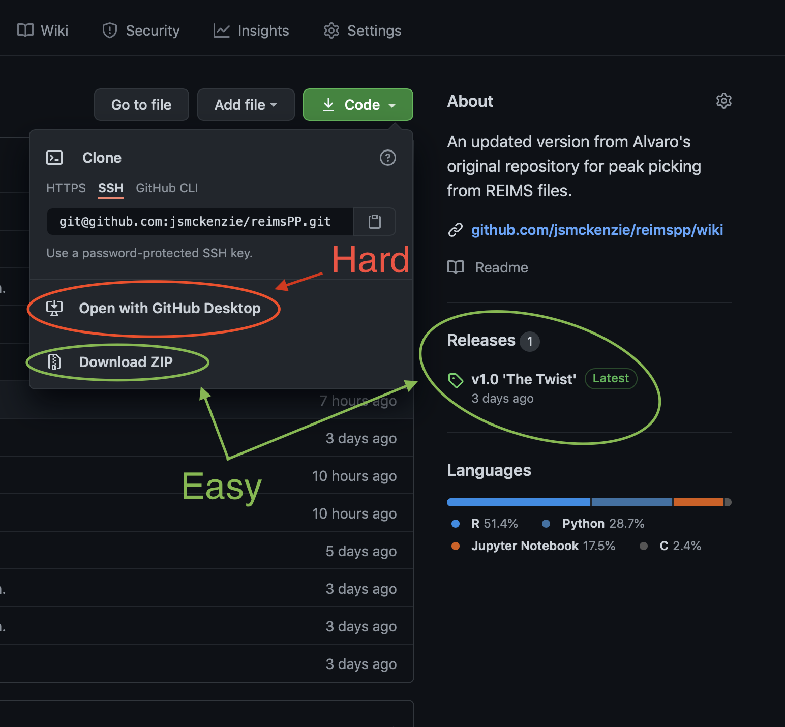
- The Easy Way
- Find the ‘Releases’ from the right hand-side toolbar and download the most recent version directly to your computer OR
- Click ‘Download’ from the green ‘Code’ menu.
- The Hard Way
- You can chose to ‘Open in Github Desktop’ so that you can get the very latest updates. This is not recommended unless you are familiar with Github.
R packages
The functions used in the R part of the pipeline depend on very specific package versions, many of which can no longer be downloaded from CRAN (which is where most of them are managed). These packages are not included in this Github repository (because they occupy a lot of space), but instead downloaded via a link found in the README. When you download this code, you should add the packages folder directly into this repository’s folder.
There is a Python function called Check_R_Packages.ipynb which you can run and it will tell you if any packages are missing / incorrect.
Other software
In addition to the two downloads mentioned above, you will need to download a few other things. These are mentioned in the Install section.
Install
Requirements
In addition to this code and the packages folder, you will also need:
- Windows (a requirement for MassLynx)
- MassLynx (a requirement for reading the raw files)
- Find a copy on the Z drive for your version of Windows
- An installation of Python 3 (more details below)
- R, Rtools, RStudio (more details below)
Python
In addition to the full-sized Conda suggested, you may also wish to consider Miniconda which is discussed in the next section.
 There may be a few ways to get the Python environment working, but this is the method that I used and should be able to help with.
- Install Anaconda from here and select the 64-bit graphical installer for Windows
- Run Anaconda Navigator (Anaconda3) from your Start Menu
- Launch JupyterLab (or Jupyter Notebook if you wish)
- Alternatively, you can run the Powershell, change drive if you have downloaded this code elsewhere (e.g. by typing
E:) then type jupyter lab or jupyter notebook
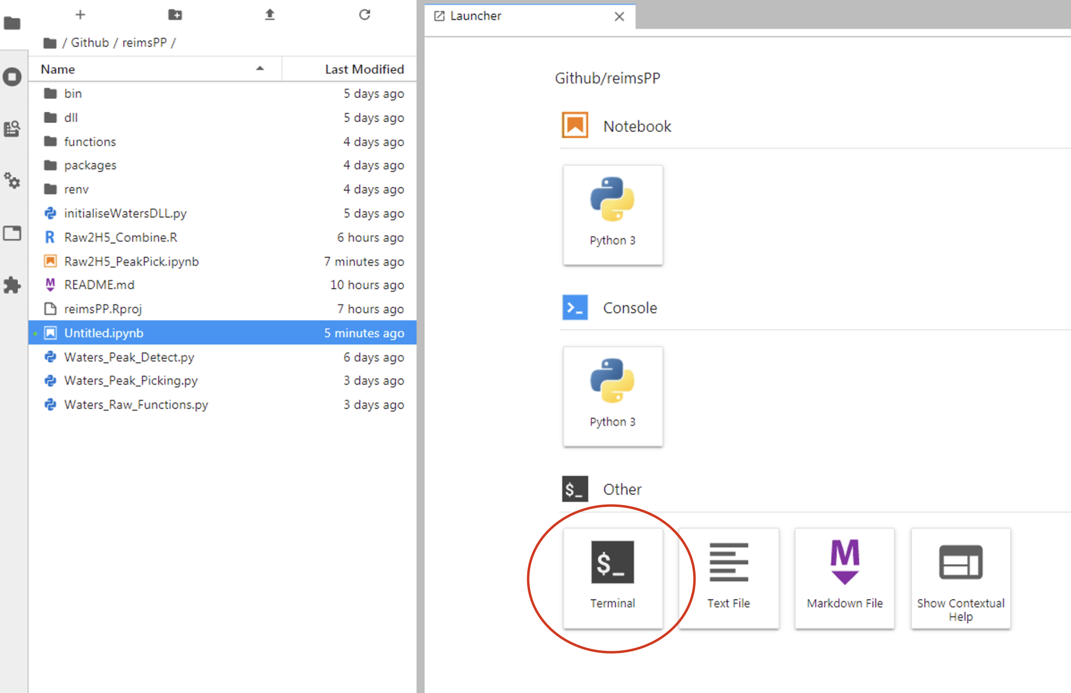
- From the main screen, open a new Terminal. Where it says (base) PS E:> or similar type the following commands one at a time, answering
y as required. Note that the # symbols are comments and shouldn’t be typed
# This creates a new environment called 'rawh5'
conda create --name rawh5 python=3.9.2

# Activate this environment
conda activate rawh5

# Install all of these packages
conda install scipy h5py numba numpy pandas pywavelets matplotlib scikit-image scikit-learn statsmodels
You can, of course, provide an alternative environment name other than rawh5. Should you ever forget what you called the environment, you can get a list of the available environments with the following command: conda env list.
That should be all that is required to install the Python environment. When you come back to it from now on, you should only need to type the following command into the Terminal: conda activate rawh5 (or whatever you called your environment).
Python via miniconda
Conda is a larger package manager that installs a lot of surplus stuff onto your computer. Instead, Miniconda might be more useful but only if you are familiar with the command line as much of the visual parts of Conda are not available. You can find a recent version from here. Once installed, open Anaconda Prompt (Miniconda3) from the Windows start menu and follow the code example above to create an environment. You may also wish to install either Jupyter Lab or Notebook (as these won’t be installed by default, unlike with Conda).
R & RStudio
These are the same requirements from Alvaro’s original pipeline, which exclusively used RStudio. Implementations of R itself, and R packages, can change quite considerably from version to version. It is because of this that these instructions are quite rigid to ensure that the correct packages are installed. Note that if you already have a working RStudio installation, you do not need to complete these stages.
- Download and install R version 3.4.4 from here
- Download and install RStudio
- It is not recommended to install RStudio from within Anaconda
- Download and install Rtools
- Open RStudio and ensure that the version listed at the top of the console is 3.4.4
- If not, you must change it via
Tools > Global Options
- In the files browser (typically bottom right panel), navigate to the repository folder, e.g. E:/Github/reimsPP/
- Run the setwd command:
setwd("E:/Github/reimsPP/") or equivalent for your computer
- Create a Project, using the button in the top right corner: New Project > Create in Existing Directory
- When completed, click on the .RProj file in the Files tab within RStudio
- In the pop-up, click Environments and tick the renv box
- Install additional packages as required
- Now install packages, one line at a time, using the following commands. Ensure that you have already downloaded the various packages (see README) and placed these in the repository folder.
# This command ensures that RStudio looks in the _packages_ folder
.libPaths("./packages")

# Each of the following commands installs a single package. Verify it has successfully been installed
install.packages("MALDIquantForeign")
install.packages("doParallel")
install.packages("iterators")
install.packages("reticulate")
install.packages("plotly")
install.packages("htmltools")
install.packages("shiny")
install.packages("dplyr")
install.packages("tictoc")
If you encounter any errors during the installation of these packages in R, please return to Python and run the function called Check_R_Packages.ipynb. This should identify any problems with missing packages, or incorrect versions. If any issues are highlighted, please download those packages from the shared folder and try again.
Run
You’ll need to run the Python code in order to perform the pre-processing of the files. The final output from the Python code is then used by the R code to align the files, perform across file peak matching and generating a csv file for statistical analysis.
In addition the ‘main’ Python and R files, there are two additional files which might be some use…
Check_R_Packages.ipynb
This Python notebook can be used to identify if you have the correct R packages installed, as specified in this wiki.
H5_File_Checker.ipynb
Use this file after the Python preprocessing to see if you have managed to successfully process all of the files. For certain reasons, some files may not have fully processed (e.g. no peaks detected), and this notebook allows you to write a new metadata file without these failed files, and this new file can be used in the R pipeline without causing crashes.
Python
Activate environment
You’ll need to launch Anaconda and your Jupyter installation of choice, and then proceed to activate the environment that you created previously. In the Terminal type conda activate rawh5 or similar, and if successful the prompt should change from (base) to (rawh5).
Open notebook
The file to open and edit is called Raw2H5_PeakPick.ipynb. Within this file, you will need to navigate to the first editable cell and update the parameters accordingly. Descriptions for each are given below.
Edit parameters
metadataName = 'C:/Path/To/Metadata.csv'
Specify the exact or relative path to a metadata (CSV) file. Exact paths begin with the drive letter, (C:/REIMS_PP/Results/), and are recommended due to their lack of ambiguity.
rawPath = 'Z:/Path/To/Raw/Data/'
Location of the raw files. They should be in one single folder and not nested.
resPath = 'J:/Folder/For/Results/'
A folder into which the results will be saved.
method = 'average+filtering2' default
'average+filtering2': average scans and filter noise using FFT with more levels of noise detection'average+filtering': average scan but doesn’t filter noise. Only use this option when you have problems with the filtering algorithms with your data'convert': this is not part of Alvaro’s original pipeline. Instead, it simply reads the raw files and exports the chosen scans to an H5 file. This option is not compatible with further analysis in the RStudio pipeline.
scans = 'csv' default
'csv': this options uses the start/end scans as specified in the metadata CSV'all': only recommended as part of the 'convert' option above, this will cause problems with the RStudio pipeline
smooth_input = 19 default
This is the parameter used for smoothing the interpolated spectra.
step_size_input = 5 and mz_step_input = 5 defaults
These are used as interval sizes for determining the noise levels in the spectra. It is recommended that you leave these values unchanged.
Instructions
Alter the various parameters in the first editable cell (called ‘Parameters to change’) according to the options specified above. Ensure that the spelling is correct and that there are no errant spaces for paths and methods.
Once these are correct, you can run each cell in turn and the results should be output to the results folder that you specified.
If you encounter any interesting errors/bugs/etc please log them in the Issues tab in the toolbar at the top.
RStudio
Open RStudio
Open this and ensure that the version of R being used is 3.4.4. This is visible at the top of the console window. If it is another version, then you can change it via Tools > Global Options.
Change folder/working directory
Use the files browser within RStudio to navigate to the repository folder.
Alternatively, run the setwd command, as in setwd(dir = 'C:/Folder/reimsPP/')
Open pipeline
Open the file called Raw2H5_Combine.R by clicking on it in the files browser. The second section contains the various parameters that need to be defined. Edit these accordingly, being careful to ensure that they are entered as requested.
Edit parameters
rootDir = 'J:/Folder/For/Results/Final/'
Where are the processed H5 files? They are likely to be in a subfolder of this folder called ‘Final’ so ensure that you provide the path to this ‘Final’ folder. [The reason being that some intermediate H5 files are produced.]
metadataPathName = 'C:/Path/To/Metadata.csv'
As for the Python pipeline, specify the path to the CSV metadata file.
doLockmass = FALSE
FALSE: do not perform. Note the lack of speech marks ‘ ‘ around logical TRUE and FALSE commandsTRUE: perform using the m/z value specified below
lockmass_mz = 554.2615
The default m/z for lock mass correction is LeuEnk with m/z = 554.2615. This may not be suitable for your data, so check accordingly. Note that this has no effect if doLockMass = FALSE
smooth_input = 19
This parameter is not used in RStudio, and will be removed in future versions.
peakMatchTol = 50 ppm
Peak matching tolerance for assimilating peak lists from the various files together.
postprocessing = '~'
on-off: use it very carefully. On-off biomarker detection. Very easy overfitting method. Creates a profile per class and combines different classesclassification: doesn’t take into account classes to build the list of peaks. More peaks in the final profile.
Instructions
Once you have edited the parameters in §2 as required, you can start to run the subsequent sections. Work down each one, the next being to load the dependent packages.
Whilst intermediate outputs are saved in case of problems, it is expected that the entire pipeline is completed in one session.
The ‘final’ result, in §9, is a CSV file called ‘matrix_for_postprocessing.csv’. This should be saved in the results folder, and is ready for further analysis using other resources (there are no statistical resources included in this repository).
Run summary
The Python and RStudio pipelines work independently of each other, so you can complete them at separate times. Once you have generated the H5 files using the Python pipeline, then you can change certain parameters within RStudio without having to return to the Python code.
No substantial modifications have been made to the code with respect to Alvaro’s original implementation. This was confirmed by comparison of CSV files from the original pipeline and this newer implementation.