| Home | 1D MS | Imaging (single) | Imaging (multiple) |
MSImageMulti
Open the workflow script flowMSImageMulti.m. This file details how to import the various files and then perform statistical analysis. Only files that have been processed using the imzmlProc repository are supported, which also requires that they have been annotated and coregistered as well.
Load instance
To load a list of files, use the following basic command to return m, an instance of the MSImageMulti class (you can call it whatever you like).
m = MSImageMulti('path',path,'files',files);
The various input parameters are detailed in the table below. Append these name/value pairs to the command above when loading any instance.
| Name | Value(s) | Description |
|---|---|---|
path |
string '/Path/To/Files/' |
Folder containing all of the files. |
files |
cell array, e.g. {'File1.mat','File2.mat'} |
List of all file names including extension. |
names |
cell array, e.g. {'F1','F2',...} |
A list of shorter names, which is useful when the file names are excessively long. |
excludeBG |
logical true,false |
If true then no annotated background pixels will be imported. |
desc |
string, e.g. 'Exp. 1' |
Optional text string to provide an identifier/name to the object. |
classes |
cell array, e.g. {'cancer'} |
Optional cell array to import only the specified files. This takes precedence over excludeBG so background pixels won’t be imported if not explicitly listed. |
meta |
table | A table which contains additional information for each file. Further information on creating the table is below. This allows additional information to be used for classification and plotting. |
Metadata
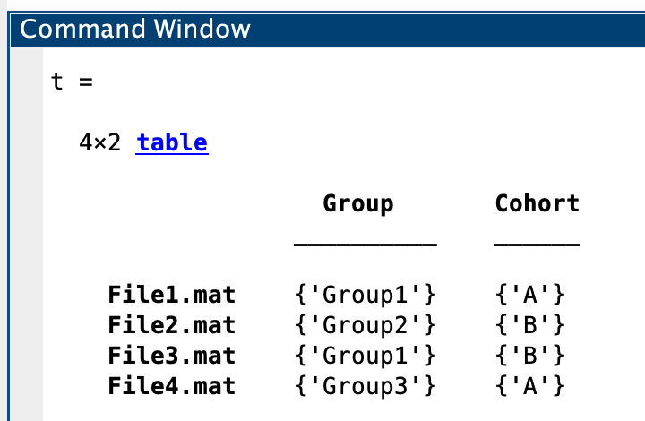
If you wish to include further information in addition to the pixel-based annotations, you can do so via a table, which is structured as below.
fileNames = {'File1.mat';'File2.mat';'File3.mat';'File4.mat'}; % list of file names (including extension)
meta1 = {'Group1';'Group2';'Group1';'Group3'}; % information matching files in `fileNames`
meta2 = {'A';'B';'B';'A'}; % additional metadata information
metaNames = {'Group','Cohort'}; % names for each of the metadata variables

% Create the table
meta = table(meta1,meta2,'VariableNames',metaNames,'RowNames',fileNames);
Statistical workflow
The following steps in the workflow are described, which must include normalisation (even if 'none' is selected).
Normalisation, transformation, batch correction
Specify one or more methods for performing normalisation and transformation. The operations are performed sequentially, thus a call of m.normalisetransform({'log','norm2'}) will produce different output to m.normalisetransform({'norm2','log'}). Performing batch correction via Combat is sufficient and does not need to be paired with other methods. Currently supported methods are:
| Value | Description |
|---|---|
'tic' |
Scales by the total intensity of each spectrum. |
'norm2' |
Scales by the Euclidean sum of each spectrum. |
'log' |
Performs log10 transformation. |
'pqn' |
Median fold change normalisation. |
'batchmedian' |
File-based batch correction using average spectra from each file. |
'combat' |
File-based batch correction using Combat, with additional options such as relating to log transformation (see below). |
'none' |
Performs no operation, but can be used to leave data as is but move on. |
Additional options
A few additional options can be specified as name/value pairs. Note that the file name is used as the batch information and there is no need to explicitly provide this.
| Name | Value(s) | Description |
|---|---|---|
'offset' |
number, e.g. 5.4 |
Provide a fixed offset for transformation. This is used during the 'log' method mentioned above, rather than during any batch correction stage. |
'combat_logmethod' |
{'global'},'local','none' |
Specify whether the data is log transformed prior to batch correction. The global approach (the default) determines a single offset across all files. The local method determines a custom offset for each file to be added prior to transformation. |
'combat_parametric' |
{true},false |
Recommended to leave as true. |
Annotations summary
This provides a simple summary of how the annotations are split over each file. The output is printed to screen, with totals calculated across files as well as annotation labels.
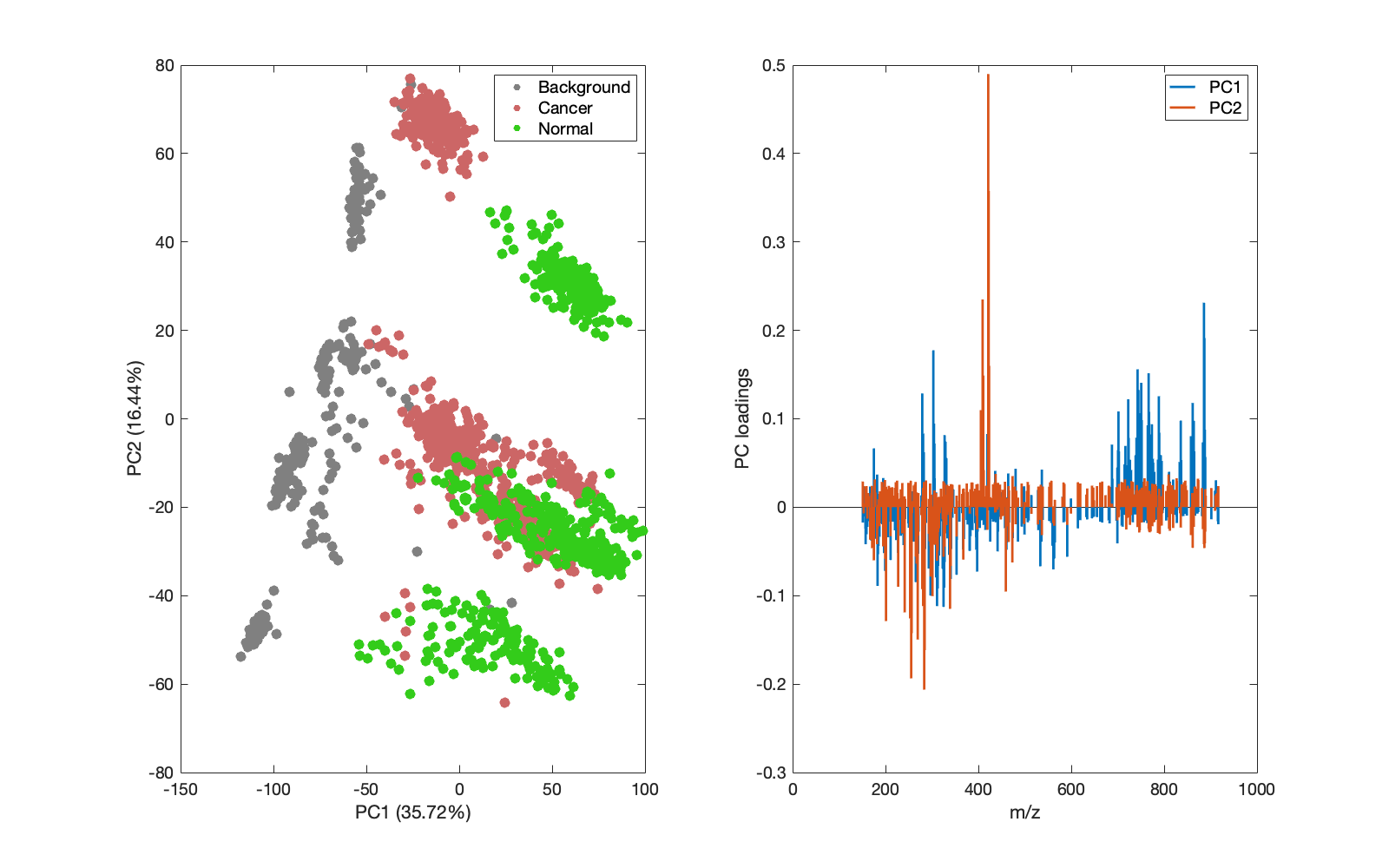
PCA
The command m = m.pcaCalculate(10); calculates the first 10 PCs for the data using the normalised/transformed data as previously determined.
To plot the results, use the m.pcaPlot(comps,scoresType,loadingType); code, which has the following inputs:
| Name | Value(s) | Description |
|---|---|---|
comps |
numeric e.g. [1 2] or [2 4 8] |
PCs to plot (specify either 2 or 3 for 2D/3D visualisation purposes). |
scoresType |
'grpID','fileID',or metadata heading |
Determine point colouring in the scores plots. |
loadingType |
'spec','scatter' |
How the loadings are displayed. |
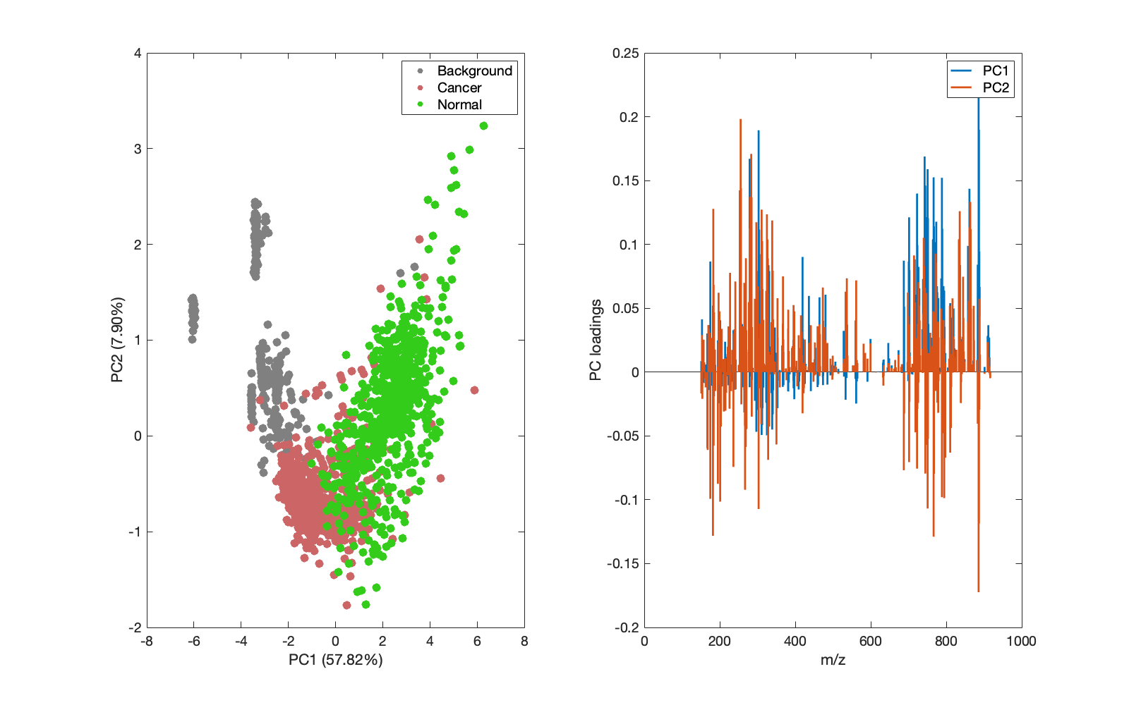
 |
|---|
Figure 1: PCA scores plot following data that was normalised by {'log','norm2'}. |
Prediction
Currently only logistic regression is implemented as a predictive/classification model. Other approaches will be implemented eventually. The standard approach is to perform cross validated prediction using a portion of the annotated pixels, typically organised on a leave-file-out basis to reduce bias. In larger cohorts and those containing multiple samples per patient, a leave file out approach is preferable.
Alternatively, model training can be performed with no cross validation, and the model can be used to predict non-annotated pixels from the remainder of the image or entirely independent samples (although not currently).
The standard call for prediction is: m = m.predict('method',method,'cv','fileID'); whereby:
| Name | Value(s) | Description |
|---|---|---|
'method' |
'lr' |
Logistic regression (no others implemented just yet…). |
'cv' |
'fileID','none', metadata table heading |
Determine how the CV is performed. Select 'none' for models to be used to predict independent samples whilst select 'fileID' to perform leave-file-out CV. |
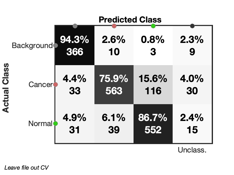
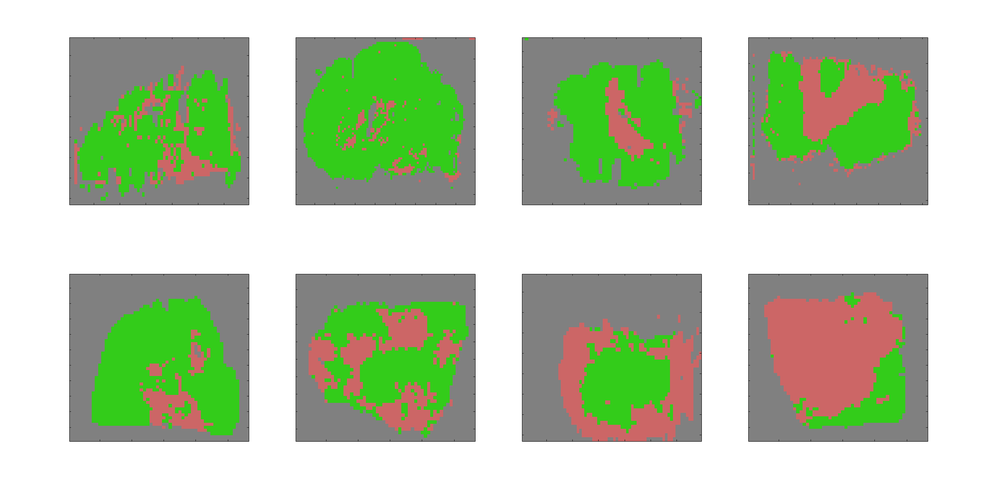
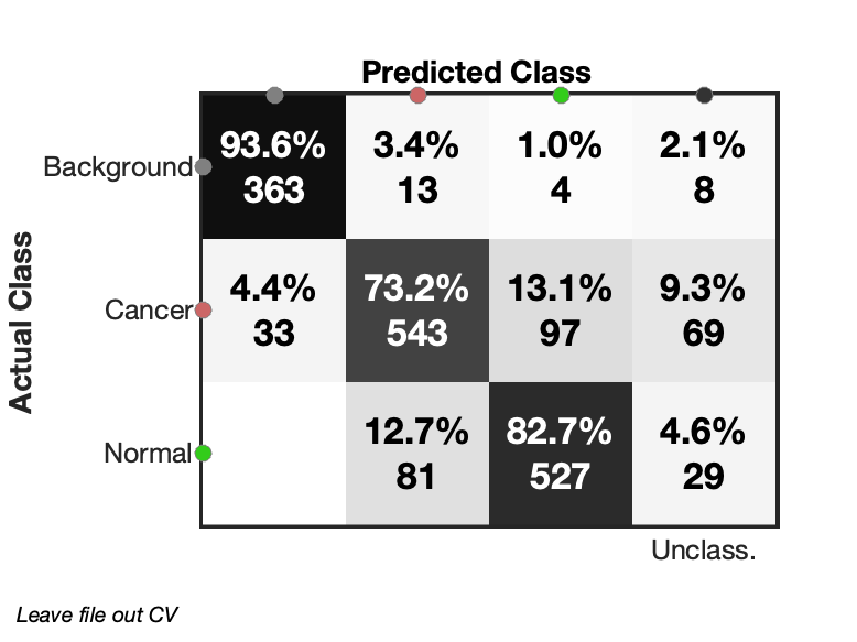
To visualise the results from 'cv','fileID' cross validated prediction, the confusion matrix can be shown by m.predictConfusionMatrix('lr'); and mini confusion matrices can be drawn with m.predictConfusionMatrixFile('lr');
 |
|---|
| Figure 2: Confusion matrix from leave file out cross validated logistic regression. Some pixels are marked as unclassified due to low probabilities. |
Projection
The data stored in the class instance is only of annotated pixels. This is for two reasons:
- Only annotated pixels can be used to train predictive models.
- Computer memory is likely insufficient to load all pixels from a cohort of files.
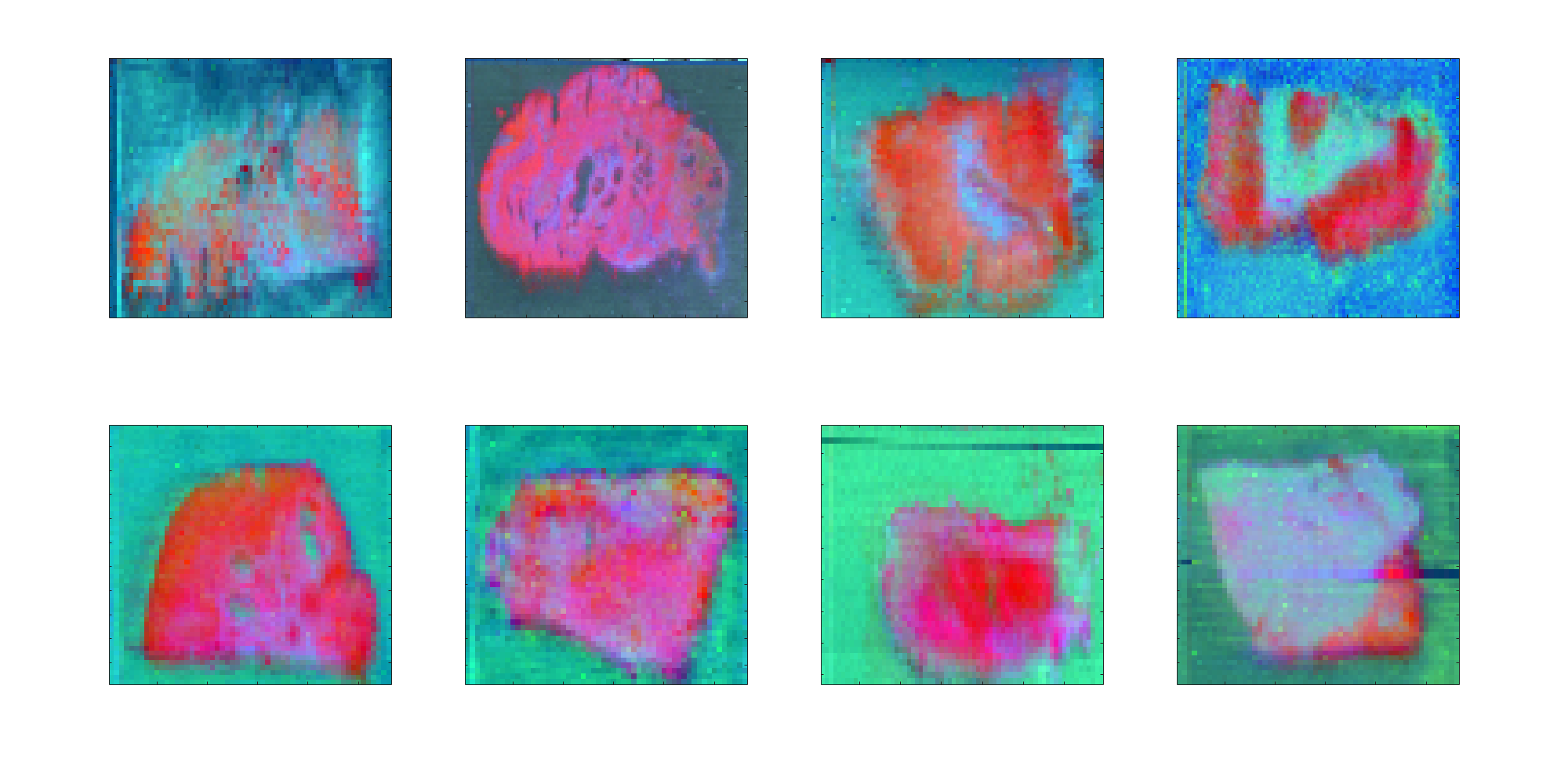
However, it may be instructive to be able to project/predict the omitted pixels from the files. The projectToImage(method) command (method = 'pca' or 'lr') allows for a model determined with the annotated pixels to be used to project/predict the other un-annotated pixels. Their results can be visualised as scores or classification images.
The results can be visualised using the following command m.projectPlot(method,type,comps); where:
| Name | Value(s) | Description |
|---|---|---|
method |
'pca','lr' |
Which method to run. |
type |
'scores','images' |
The scores can only be plotted for PCA. |
comps: |
e.g. [2 3],[1 2 3] |
To specify which PCA components are to be plotted. |
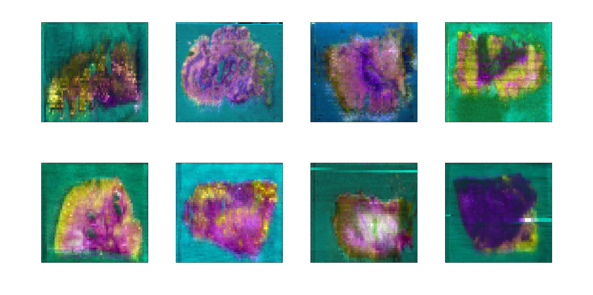
 |
 |
|---|---|
| Figure 3a: PCA scores (components 1,2,3) following projection using the PCA model. | Figure 3b: Prediction of all pixels using a hold out model determined using only the annotated pixels. |
Batch correction
Due to inconsistencies in the way data were acquired, batch correction may be useful to remove these sources of variation from one sample to the next. In some cases a simple correction might be sufficient, such as by using fold change normalisation ('batch','median'). This corrects each file according to the global average spectrum akin to median fold change normalisation and provides a single scaling factor by which to scale each observation. It is likely most effective for small (and simple) batch effects which tend to modify the intensities in a fairly even and predictable way.
For more complicated batch effects, such as for those with non uniform changes, Combat batch correction ('batch','combat') is likely to be more suitable. It uses Bayesian approaches to modify the intensities, and as each variable is scaled individually the scaled spectra will likely have a different profile.
Log transformation can be applied to the data prior to the batch correction if required. If 'global' is selected, then a single offset is added to the data prior to transformation. If 'local' is selected, then an offset is determined for each file (which is likely to vary for each file) prior to transformation.
Where Combat batch correction is applied, there is seldom any need for further normalisation or scaling, thus the normalisation stage should be performed to leave the data unchanged: m = m.normalisetransform({'none'});.
Comparison
A batch effect is visible in the PCA scores shown in Figure 1 despite normalisation and transformation. Instead, the data is batch corrected on loading, and the PCA scores are shown in Figure 4 below adjacent to those from the non-batch corrected data.
|
 |
|---|---|
Figure 4a: PCA scores with no batch correction, but {'log','norm2'} normalisation/transformation. |
Figure 4b: PCA scores with no normalisation/transformation but Combat batch correction performed with global log transformation. |
Whilst the PCA above shows noticed improvements in bringing like pixels/spectra together, the classification results from logistic regression (Figure 5) are at odds with an improved clustering in PCs 1 and 2.
|
 |
|---|---|
| Figure 5a: Confusion matrix of non-batch corrected data. | Figure 5b: Classification results using batch corrected data. |
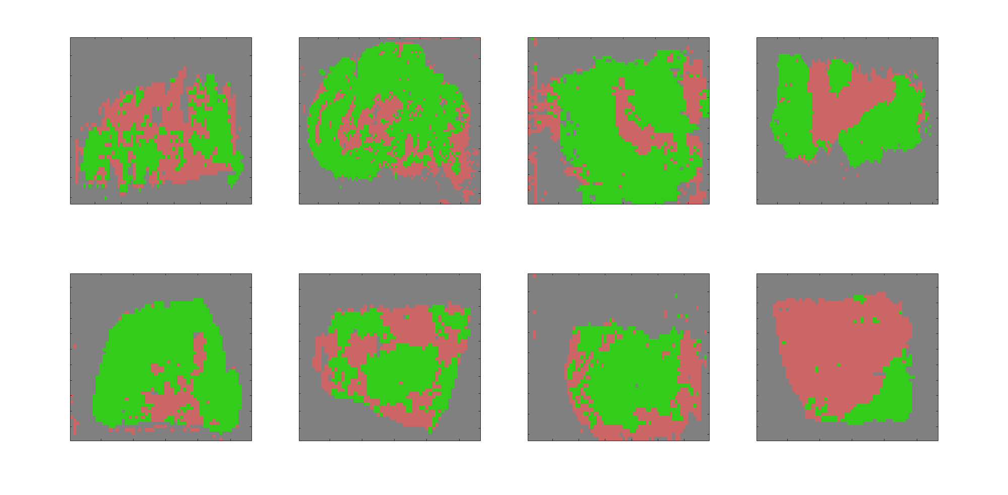
The results from projection to the full images are shown for comparison in Figure 6 and the classification results in Figure 7. These images provide no indication of whether batch correction is suitable for other datasets.
|
 |
|---|---|
| Figure 6a: PCA projections of non-batch corrected data. | Figure 6b: PCA projections of batch corrected data. |
~
|
 |
|---|---|
| Figure 7a: Predictions of non-batch corrected data. | Figure 7b: Predictions of batch corrected data. |
| Home | 1D MS | Imaging (single) | Imaging (multiple) |