| Home | 1D MS | Imaging (single) | Imaging (multiple) |
MSImage
The analysis of a single file can is outlined in the workflow flowMSImage.m.
Load instance
To load a single file, use the following command where fp is the path to the processed .mat file, and fn is its name (including extension).
d = MSImage(fp,fn);
This loads an instance of class MSImage, whose various methods can be shown by running the command methods(d). The object d can be renamed as required, but is used throughout the workflow.
Visualise tissue
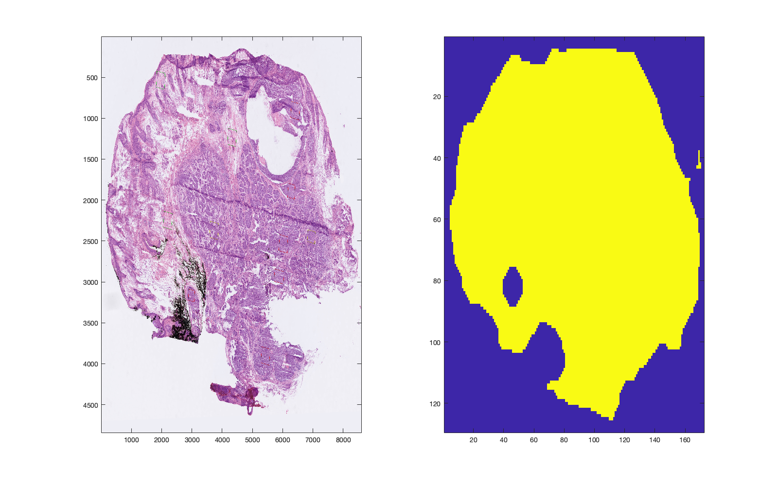
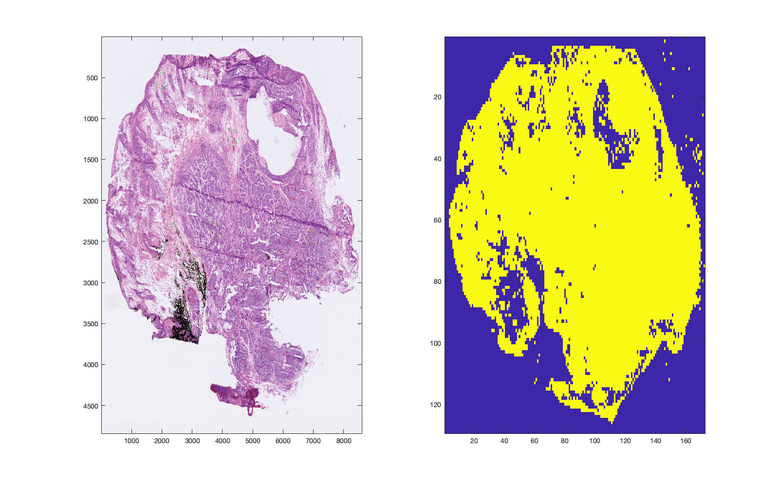
The next section of the workflow is to visualise the tissue/background partition image. This is used in further sections to automatically identify/remove background pixels. By default, the TOBG map is taken from the coregistration stage. If this is not suitable, then an alternative background partition using the 1st PC can be performed by d = d.dettobg(method);, whereby method is set to 'pc'. To revert to the previous TOBG map, set method as 'coreg'.
 |
 |
|---|---|
| Figure 1: Tissue/background map determined during the coregistration stage. | Figure 2: Tissue/background partition determined using PC1 as an input to Otsu thresholding. |
Normalisation and transformation
Specify one or more methods for performing normalisation and transformation. The operations are performed sequentially, thus a call of d.normalisetransform({'log','norm2'}) will produce different output to d.normalisetransform({'norm2','log'}). Currently supported methods are:
'tic': scales by the total intensity of each spectrum'norm2': scales by the Euclidean sum of each spectrum'log': performs log10 transformation. The offset can be provided as an optional name/value pair as inm.normalisetransform({'log','norm2'},'offset',5.9). If not provided, it will be calculated automatically'pqn': median fold change normalisation'none': performs no operation, but required prior to progression to other sections
Principal components analysis
The PCs can be calculated by [d] = d.pcaCalculate(numComps,excludeBG); where numComps is an integer specifying the number of components to calculate, and excludeBG is either true/false to determine if the PCA should be performed with or without background pixels.
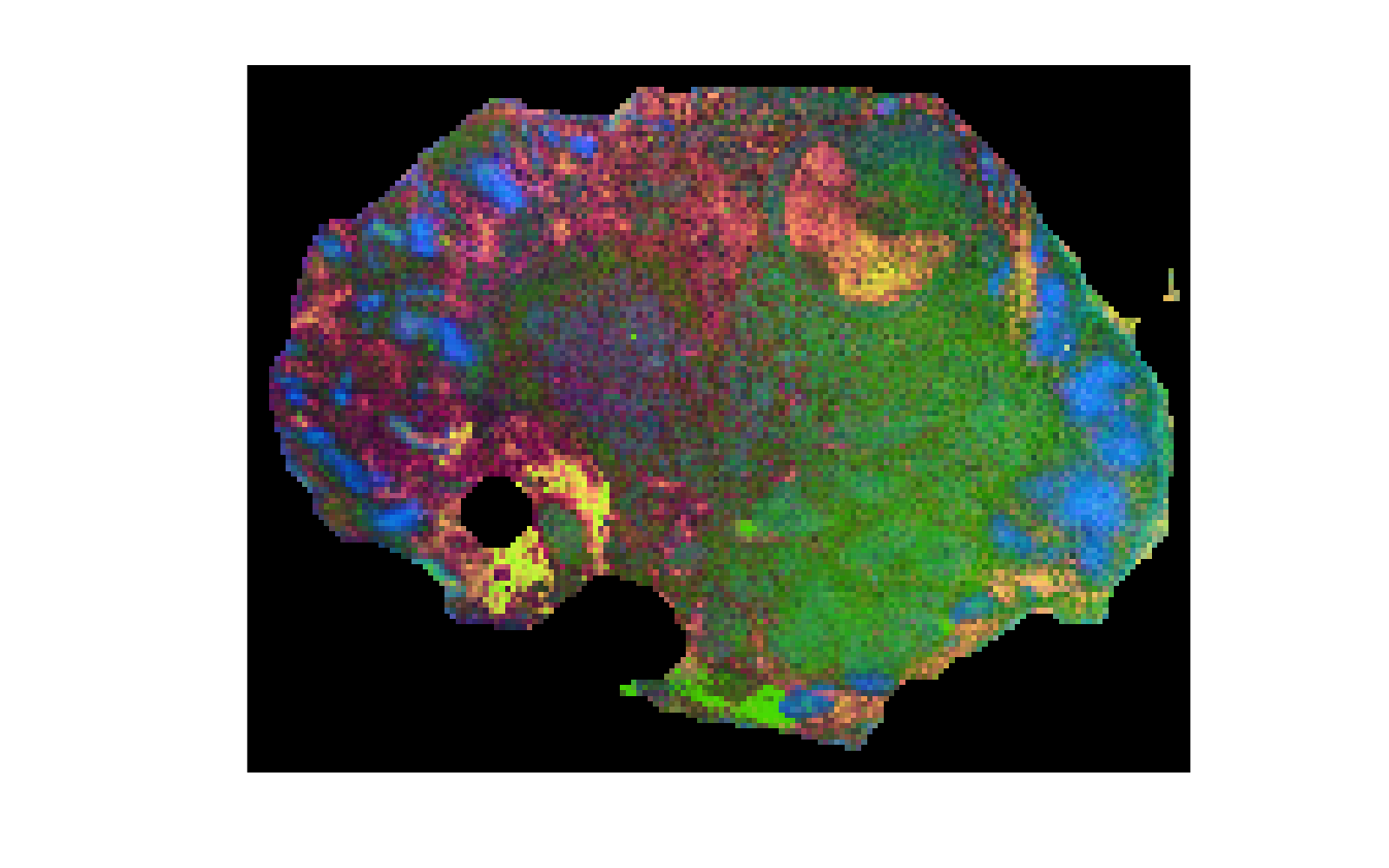
PC images can be plotted in a single figure as either single components (plotComps = 1) or three components (plotComp = [1 2 3]) as an RGB image: d.pcaPlotImage(plotComps);. The first three components for an example file are shown below…
 |
|---|
Figure 3: PC plot showing components 1-3 as a scaled RGB image. Intensities of each component are scaled between 0 and 1. Note that the background pixels are not included as excludeBG = false. |
 |
|---|
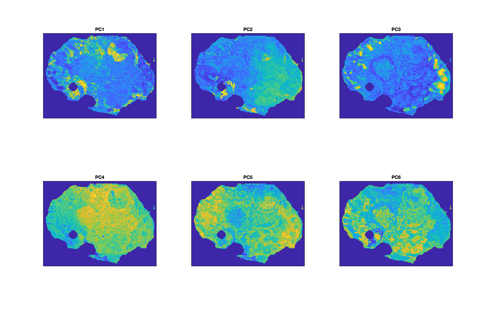
Figure 4: Array of PCs 1-6 generated with the command d.pcaPlotImageArray(6);. |
Predictions with cross validation
A cross validated model is generated using only the annotated pixels. The results from this model provide an estimate of the strength of the data (spectra + annotations) for predictive purposes, such as to be able to predict entirely independent datasets.
The simple command is:
[d] = d.predictCV('method',method,'numPCs',numPCs,'useBG',useBG,'cv',cvMethod);
The options for each name/value pair are as follows:
| Name | Value(s) | Description |
|---|---|---|
method |
'lr' |
Currently only logistic regression is implemented. |
numPCs |
integer, e.g. 3 |
Specify the number of PCs to use as a data reduction method. To use the non-reduced dataset, specify this value as 0. |
useBG |
logical, true,false |
Setting this to true includes a random subset of background pixels into the analysis. Note that if the image already has annotated pixels, it will include another subset of background pixels. |
cv |
'lro','lpo','kfold' |
Leave region out CV only works where there are multiple annotations for each type. Leave pixel out CV is slow in situations where there are more than 100 pixels. K-fold annotation is the alternative where LRO or LPO are not suitable. |
k |
integer, e.g. 10 |
Specify the number of folds for k-fold cross validation. The default is 10. |
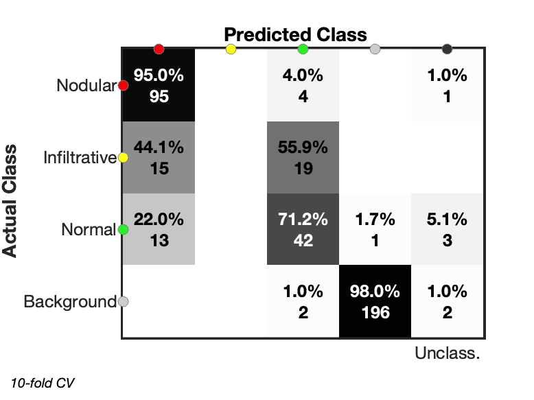
The results of cross validated predictions can visualised as either a confusion matrix or an image, as shown in below.
useBG = true |
useBG = false |
|---|---|
 |
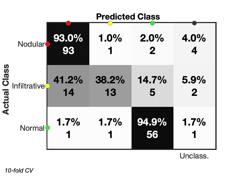 |
| Figure 5a: Confusion matrix showing classification results with included background pixels. Not all pixels could be classified with a final column listing the unclassified pixels. | Figure 5b: Confusion matrix shown for pixel classification without included background pixels. As before, certain pixels are unable to be classified. |
 |
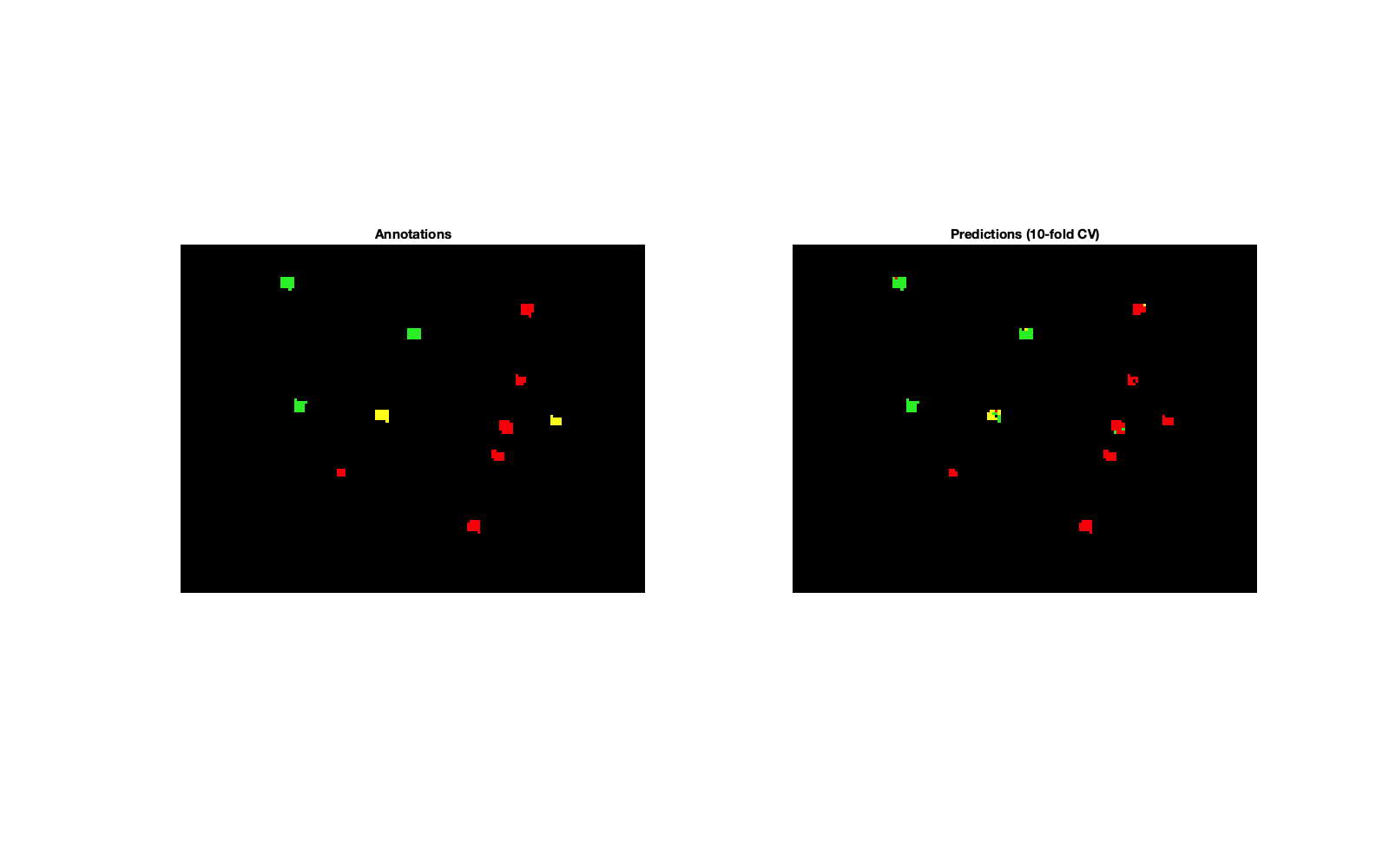 |
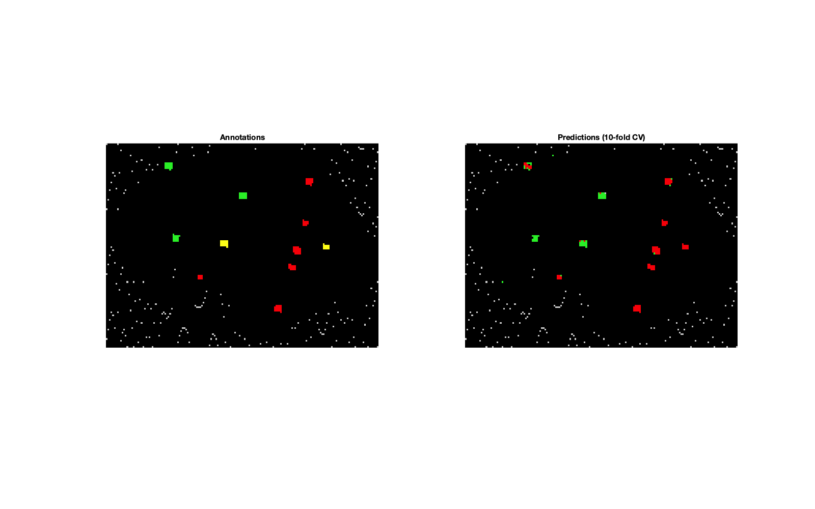
| Figure 5c: Image showing annotations and predictions based on the annotation colours shown in the confusion matrix. 200 background pixels have been included based on the TOBG partition. | Figure 5d: Classification image when no background pixels are included. |
Predictions across remaining pixels
The previous section trained a cross validated model amongst the annotated pixels, and thus provides an estimate of how well the annotated spectra are capable of predicting other pixels. This section uses all annotated pixels to train a classification model and then predicts all pixels within the image.
The command [d] = d.predict('method',method,'useBG',useBG); follows previous syntax in terms of method and the addition of background pixels if none were annotated.
 |
 |
|---|---|
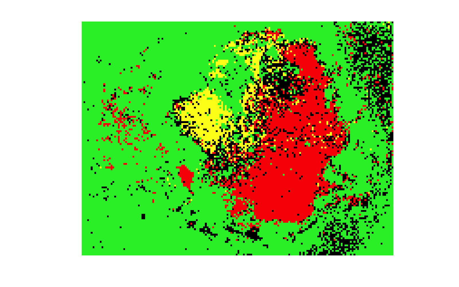
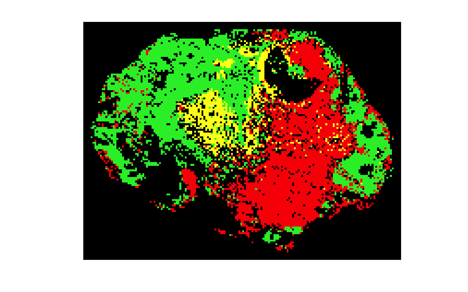
Figure 6a: Prediction results when useBG,false. As there is no background class, a lot of the background and low intensity pixels are classified as one of the other tissue types. |
Figure 6b: By including a subset of the background pixels, a more realistic classification can be achieved with logistic regression. |
Univariate statistics
The annotated pixels can be used to determine statistically significant differences in intensities with the following command [d] = d.univariate(method);. Valid values for method are 'anova' or 'kw'/'kruskal-wallis'. This method outputs nothing to screen but the top k variables can be seen in the table output by d.univariateTopVariables(k);.
The table resembles that shown below, with mean and median values calculated for each annotation group (here A, B, C). The table is sorted by ascending q value, i.e. most significant at the top.
| m/z | p | q | A-Mean | B-Mean | C-Mean | A-Median | B-Median | C-Median |
|---|---|---|---|---|---|---|---|---|
| 684.81 | 1e-10 | 1e-09 | 1.6890 | 2.3144 | 2.1498 | 1.7042 | 2.3444 | 2.1805 |
| 246.10 | 1e-09 | 1e-08 | 1.4443 | 2.0215 | 1.8808 | 1.4803 | 2.0517 | 1.8917 |
| ~ | ~ | ~ | ~ | ~ | ~ | ~ | ~ | ~ |
Particular features can be visualised by ion image plots or boxplots. Ions need to be provided as indices (rather than m/z values) to these functions, but the command idx = d.getIndex(ions); (where ions = [255.23 256.23 ...])) will determine the requisite indices.
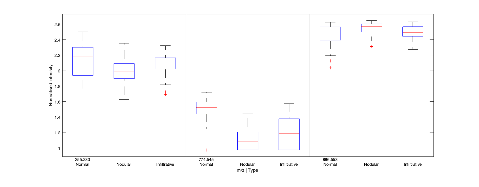
The boxplots in Figure 7 were generated as follows: d.plotVariables(idx,'boxplot','anno'); which draws plots of the annotated pixels. Ion images for 1 or 3 ions can be drawn using the ionPlotImage method.
 |
|---|
| Figure 7: boxplots of 3 variables grouped by m/z value and annotation label. |
tSNE
This is a non-linear dimensionality reduction technique. There are plenty of options and settings that may be modified by amending the structure returned from running tsneOpts = d.tsneOptions;, however do not edit them within the MSImage class file. Type doc tsne into the command line for help regarding the options.
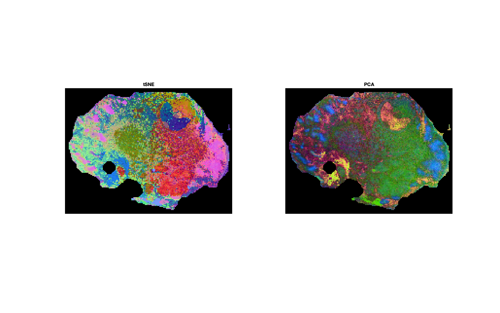
Visualise the embeddings by running d.tsnePlotImage(plotComps,showPCA) and specifying plotComps = [1 2 3] and showPCA = true for a side-by-side comparison.
 |
|---|
| Figure 8: comparison of the first three components from tSNE and PCA. |
Clustering
Simple k-means clustering can be applied to the PCA or tSNE data. The following command requires the number of clusters, k, and input data (type = 'pca' or 'tsne') to be specified: d = d.kmeansClusters(k,type);.
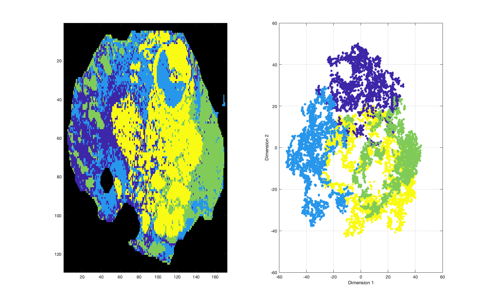 |
|---|
| Figure 9: k-means clustering of the tSNE embeddings into 4 clusters. The embeddings are shown in x-y-z space, so the right-hand axes can be rotated as required. |
| Home | 1D MS | Imaging (single) | Imaging (multiple) |