Home-Download-Recalibrate-Pre-process-Annotate1-Annotate2-Coregister-Statistics

Annotate

This page details how annotations can be extracted from H&E images which have the annotations drawn on them. These normally are rectangular regions (other shapes supported) with an outline colour that is indicative of the annotation (e.g. red = cancer). There should be no large black regions drawn in and no text. Also ensure that the colours in the images are consistent across files in a cohort.

For images which are without drawn-in annotations, i.e. untouched H&E images, then the alternative annotation section allows for regions to be drawn in prior to the coregistration stage.

Objective

The aim of the UI is to be able to identify annotations regions in H&E images to be marked and saved. These annotations will then be coregistered in the next stage of the revised workflow.

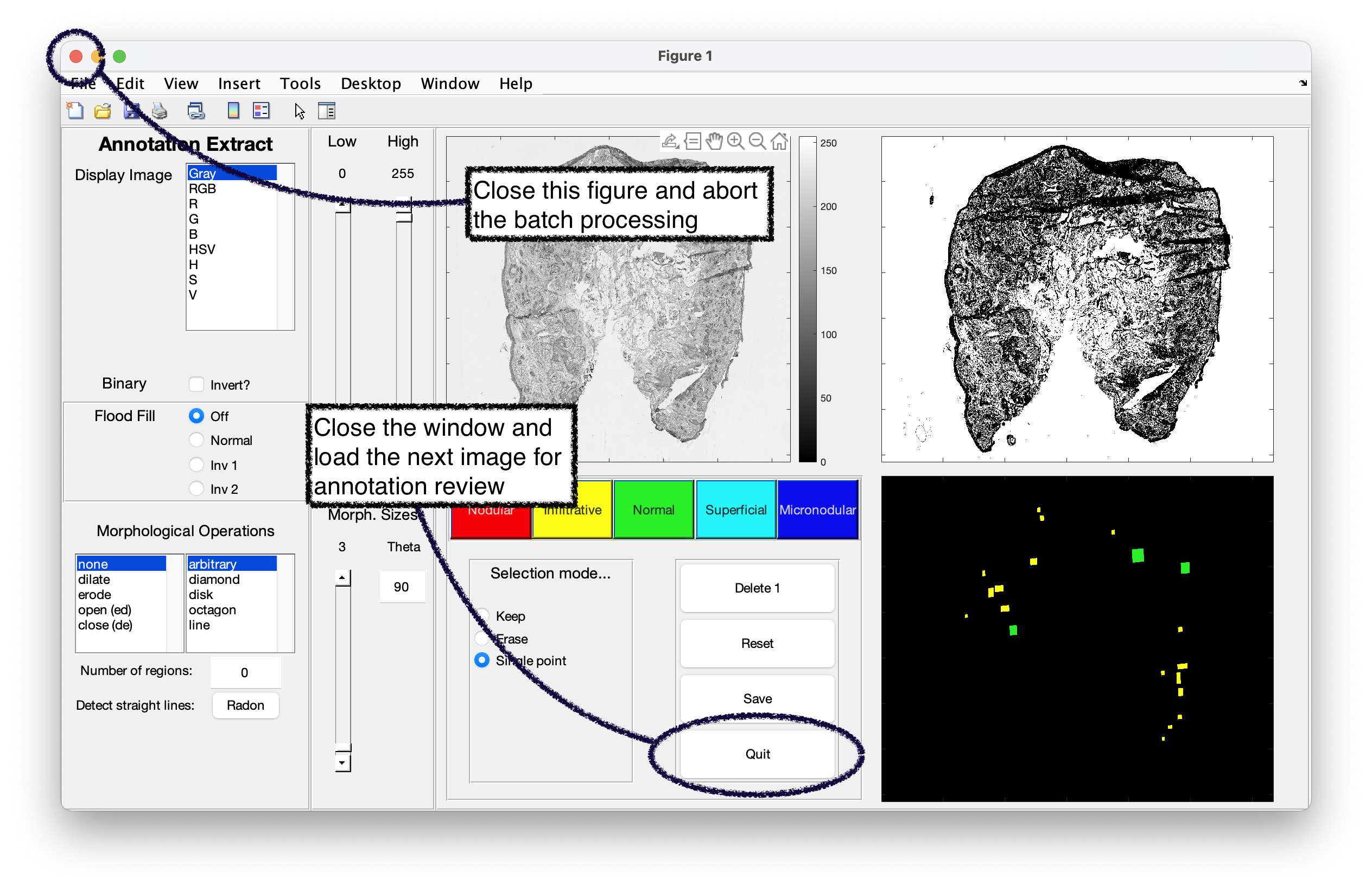
The interface allow the image to be shown in different ways, and the thresholds changed in order to identify the annotations within. These need to be filled regions of white pixels in the binary image, which are then manually added to the annotation mask shown in the bottom right axes. Once completed, the annotations are saved and the window can be closed. In batch mode, using the Quit button loads up the next image whilst closing the figure (❌) will abort the batch processing.

Single file operation

The function to help extract the annotations from a single image is called AnnoExtract and it has one mandatory input and various optional input arguments. By default certain annotations are used, but you can specify your own (provide names and colours) as shown below.

myAnnotationLabels = {'Normal',[0.2 0.8 0.1];...
    'Cancer',[0.8 0.4 0.4];...
    'Background',[0.5 0.5 0.5]};

AnnoExtract(img,'savePath',savePath,'saveName',saveName,'init',true,'anno',myAnnotations);

The input arguments are as follows:

img : the input H&E image as imported using a function like img = imread('/Path/To/File.jpg')
savePath : the default location (e.g. '/Path/To/Save/') in which to save the file (note that this doesn’t actually save the file)
saveName : the image name (e.g. '147.jpg') to be used to save the file
init : either true or false, this specified whether an initial estimate of the annotations should be made
myAnnotations : a cell array of labels and colours (see example above). Ensure that these are consistent across a cohort of files

Starting estimate

When specified with init, this option will make an initial estimate of the location of the annotations. It works effectively for certain images, but is not guaranteed for all images. When set to true the interface will launch with the estimated annotations which can be manually reviewed / edited / deleted as required.

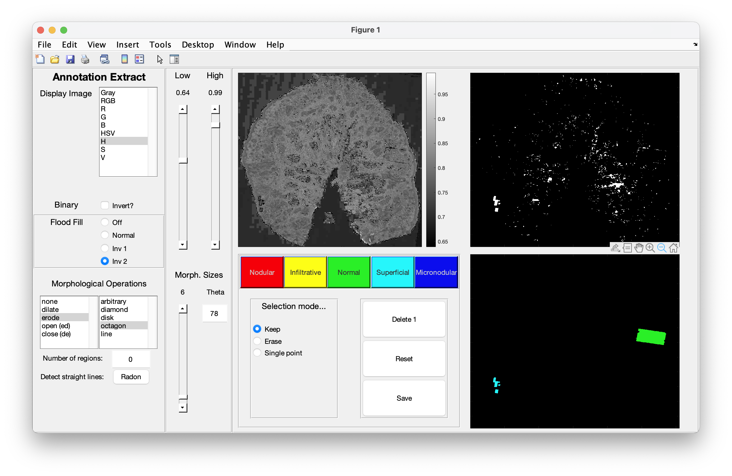
Interface

On launch, the interface resembles that shown in the figure below. This is image 147.jpg which is not well estimated by the init process. It contains a patch of cyan annotations at 8 o’clock and a single green annotation at 3 o’clock.

anno-1

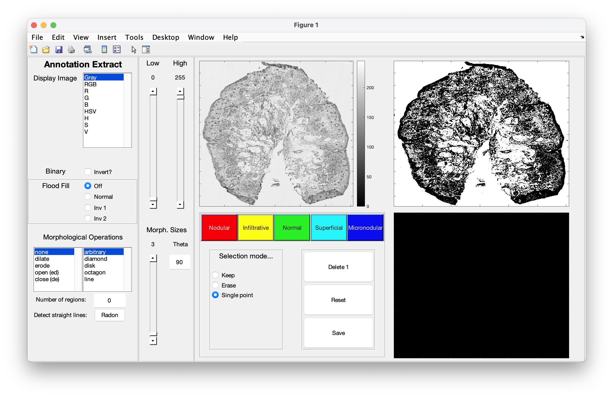
Axes

Image (top left): displays the image representation selected in the list box on the left hand panel
Binary (top right): displays the binary image determined from the selected image
Annotations (bottom right): displays the annotations determined for image thus far

Image and binary options

There are various options in this left-hand panel:

Image choice

The image can be shown as one of a series of representations: gray scale, RGB, HSV, or the individual channels of the latter two. This choice is reflected in the top left axes panel.

Binary

Although the binary is drawn by default, this option allows the binary to be inverted. This affects how the flood fill operations work so certain fills may work best with a normal image and others with the inverted binary.

Flood fill

The aim of these operations is to fill the image, so the normal fill assumes that the background is black and the tissue/annotations are black. All black pixels connected to the seed pixels (approximately the image corners) are filled white. The difference between Normal and Inv 1 is that the results are returned inverted. Inv 2 provides an additional fill functionality where the pixels within certain regions are also filled and thus rectangular annotation regions may look less noisy.

Morphological operations

These operations work on the binary image and modify the appearance of the image. They can be used effectively to remove erroneous pixels or to smooth out noisy regions of an annotation. Dilation makes pixels bigger whilst erosion makes them smaller; open and close are operations of both successively. The neighbouring list box determines the element used to filter the binary image, such as an octagon or disk. The sizes of these can be edited with the ‘Morph. Sizes’ slider in the adjacent panel.

Number of regions

This is slow process, but is useful to restrict the number of white regions especially in noisy images where the expected annotations are the largest regions of connected pixels. Leaving the value at 0 will show all regions in the binary image (i.e. no processing) but a value of n will show only the n largest regions in the image.

Radon transform

The Radon transform is used to detect straight lines in images, and can be useful in situations where one annotation can be found easily in the binary image and thus the angle(s) of the rectangle’s lines can be found. This angle is then used in the morphological ‘line’ filtering function to help smooth the detection of other lines in the image. It is at best a temperamental feature and as yet isn’t essential for any image tested thus far.

Slider panel

The adjacent panel contains three sliders and a text box.

Low

This sets the low threshold of the image shown; pixels equal to or less than the value shown are set to that value.

High

As with high, but changes the upper limit of pixel intensities. Note that for multi-channel images (RGB, HSV) the thresholds are changed for all channels equally, thus a value of 140 will set the red, green and blue maximum values to 140.

Morphological size

The slider determines the size of the filter used in the relevant morphological operation. Note that octagonal filters are changed in multiples of 3.

The text box allows the angle (theta) of the line filter to be set, which is useful for filtering partially complete rectangles (flood fill requires completely enclosed rectangles to be able to work effectively). Any operations performed using the line element performs two successive filtering operations: the first at the angle specified and the second at that angle increased by 90 degrees. These two are then combined in the displayed binary image.

Annotation panel

Drawn with colours and annotation labels, this panel allows regions of the binary image to be saved as annotations. By picking an option in the ‘Selection mode’ region and then clicking one of the coloured boxes, one or more regions from the binary image can be marked as annotations of that colour/type.

Single point : select a pixel, and all connected pixels will be marked as a single annotation
Keep : draw a closed region in the binary image and add all white pixels within that region to the annotation mask
Delete : draw a closes region and add all other white pixels to the annotation mask of that colour

Additionally, there are some push buttons:

Delete 1 : select a single region in the annotation mask (bottom right) and remove it
Reset : remove all annotations detected thus far
Save : open the save dialog to save the file
(Quit) : only in batch mode this will be visible. It is to close the figure and load the next image ready for review.

Example (147.jpg)

The following images show how the annotations can be extracted from this image.

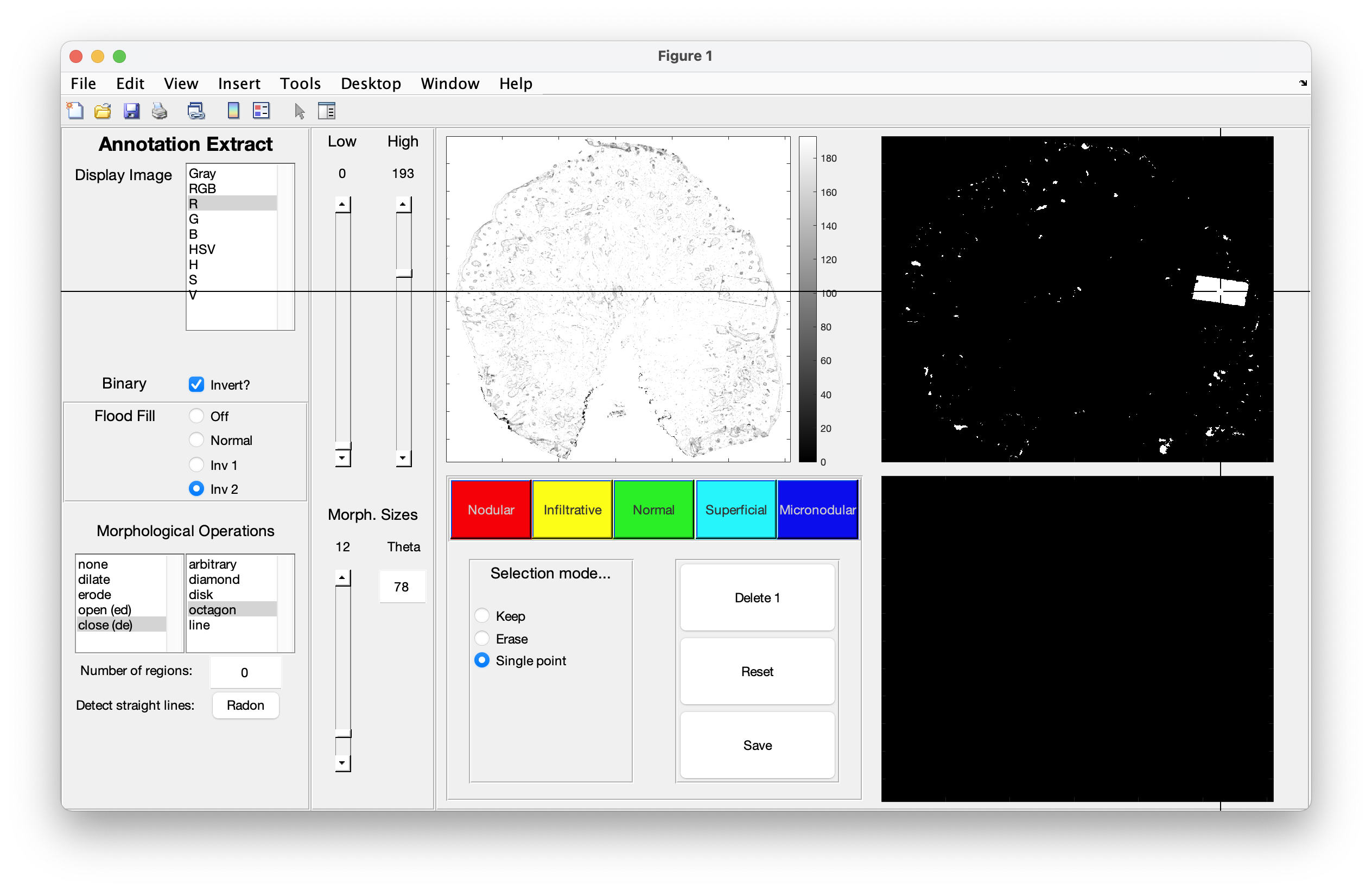
Green annotation

Using the red channel, the high threshold can be lowered to help produce higher contrast image. By inverting the binary and using the ‘Inv 2’ fill operation, the rectangle can be visualised. It is improved by using the inclose operation with an octagonal filtering element. Finally, the region is selected using the ‘Single point’ option. anno-2

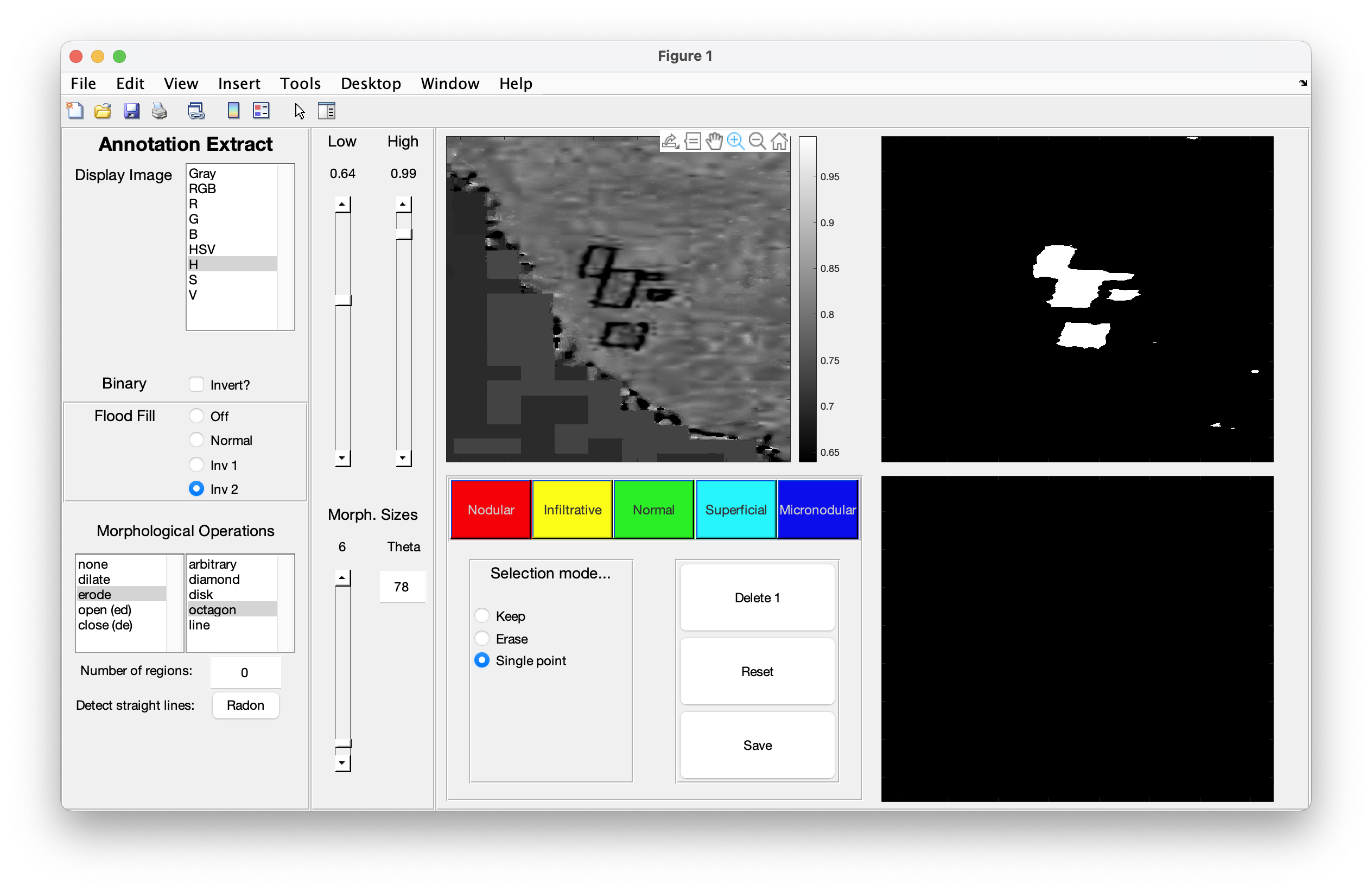
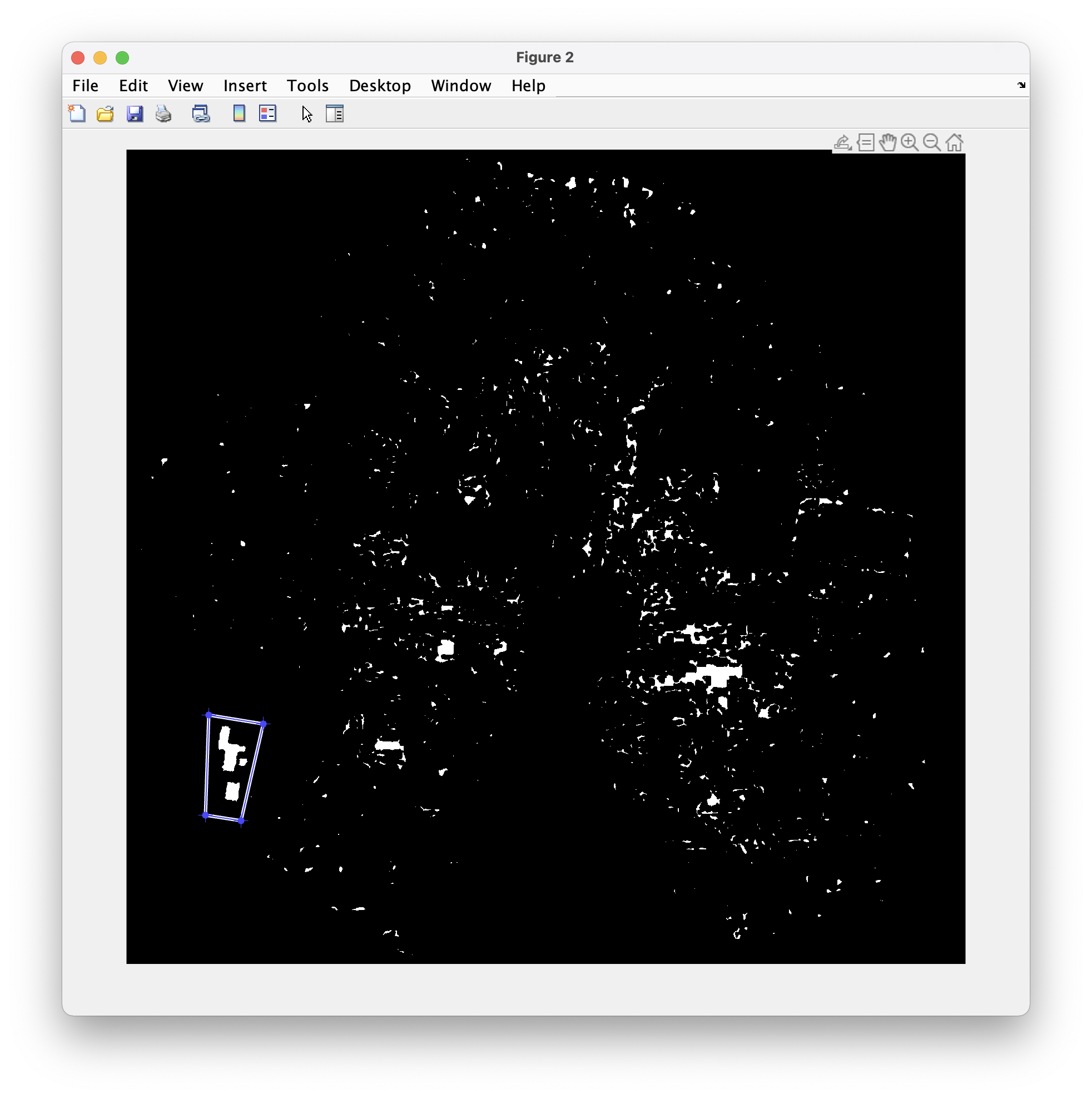
Cyan region

A high contrast hue image can be used to identify the cyan rectangles, which the ‘Inv 2’ flood fill successfully identifies. These regions are tidied up with the erode function and added to the annotation mask using the ‘Keep’ option. This draws another figure upon which the selection is made. To ‘close’ the region of interest, double click the left mouse button or right click on the polygon and select create mask. anno-3 anno-4

Final results

The final results from the two annotations are shown in the figure below. This can now be saved and the window closed. anno-5

Batch operation

The script called AnnoExtractWorkflow.m is designed to work through a folder of images that require their annotations to be extracted and reviewed. It works similar to other batch functions, where an image is loaded for the annotations to be reviewed and once complete the results are saved. The next image is then loaded and the process continues until aborted or all images have been processed.

The locations in the PATHS cell require changing to suit the location of your files:

hePath : the folder containing all of the H&E images to be reviewed
savePath : the folder in which the results are to be saved

Further options must be specified as shown below

initialEstimate = true : or false to prevent initial estimate being shown
annotationMode = 'advanced' : the alternative is 'simple' for which further information can be found here
annoType = '?' : specifies the annotations as defined in the switch annoType code block

The script will look for all images in the folder, and load each in turn for review and saving. Once the annotations have been completed for an image and it has been saved, use the quit button to load the next image. To abort processing, close the interface (❌)

anno-6