Home-Download-Recalibrate-Pre-process-Annotate1-Annotate2-Coregister-Statistics
Pre-process
Once the recalibration function has been performed, the following stages can be performed in turn. Each is briefly explained within imzmlWorkflow.m. The next stage in the pre-processing workflow is to determine the average (mean) spectrum for each image. The recalibrated mean spectra from all files are used to perform peak picking in the next stage. This is a relatively slow process for centroid mode data, and significantly slower for profile mode data.
§1 - Generate average spectra for each file
Rather than the average, it is actually the summed spectrum from each recalibrated imzml file that is determined in this section. Interpolation at a fixed m/z interval is performed (for profile mode data) because each pixel’s spectrum is unique. Centroid mode data is binned. The summary of the processing is:
- Import imzml file
- Perform recalibration using results from previous step
- Determine which pixels to consider
- Interpolate spectra to fixed resolution
- Sum all spectra
- Save
Parameters
recalPath = '': the path where the results from recalibration were saved
interpPath = '': the path into which to save the individual spectra
tobgType = 'all' or '885': in determining the spectrum, use all pixels (including background) or just those with a detected signal at m/z = 885. This assumes that 885 was used as a recalibration peak
mzRes = 0.001: fixed resolution for interpolation/binning, e.g. [400.000, 400.001, 400.002,…]
❗ recalPath, interpPath, and other such ‘results’ folders must be different locations. Files are saved to these locations using the same file name as the imzml file, i.e. all intermediate stages resulting from ‘BCC7.imzml’ will be saved as ‘BCC7.mat’, regardless of which stage is being performed. Thus it is important to specify different folders and to not move files around the folders.
Output
The (recalibrated) average spectra are saved to the folder specified.
§2 - Import the average spectra
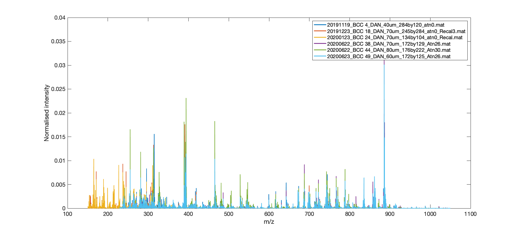
Import all of the average spectra found in the ‘interpPath’ folder. Its second argument is a logical TRUE or FALSE which determines if a figure of these spectra is drawn. The output ‘data’ is used in the subsequent peak picking function. Note that some files may have different m/z ranges due to differences in acquisition. An example figure of 6 spectra is shown in the figure below.
§3 - Peak picking
Peak picking is performed on the (mean) average of the individual spectra. Only the m/z range that is common to all files is processed. This single grand mean spectrum is smoothed with Savitzky-Golay filtering using a Gaussian window, the size of which can be modified. A threshold is determined to attempt to differentiate between noise and genuine peaks, and a multiplier is set in this section to modify the number of peaks that are picked.
Input
Aside from the parameters detailed below, the function requires the output from §2 as well as the m/z resolution from §1.
Parameters
smoothWindow = 21: this is the size of the Gaussian function used to perform Savitzky-Golay filtering. By default it uses a 21-point window, i.e. with its maximum at the 11th point
multFac = 1: the greater the threshold, the more peaks are included. A factor of 1 results in the default number of peaks, as shown in the figure below
Output
The ‘pks’ structure contains the list of peaks found in the average spectrum. It is used as one of the inputs of the next section.
Figures
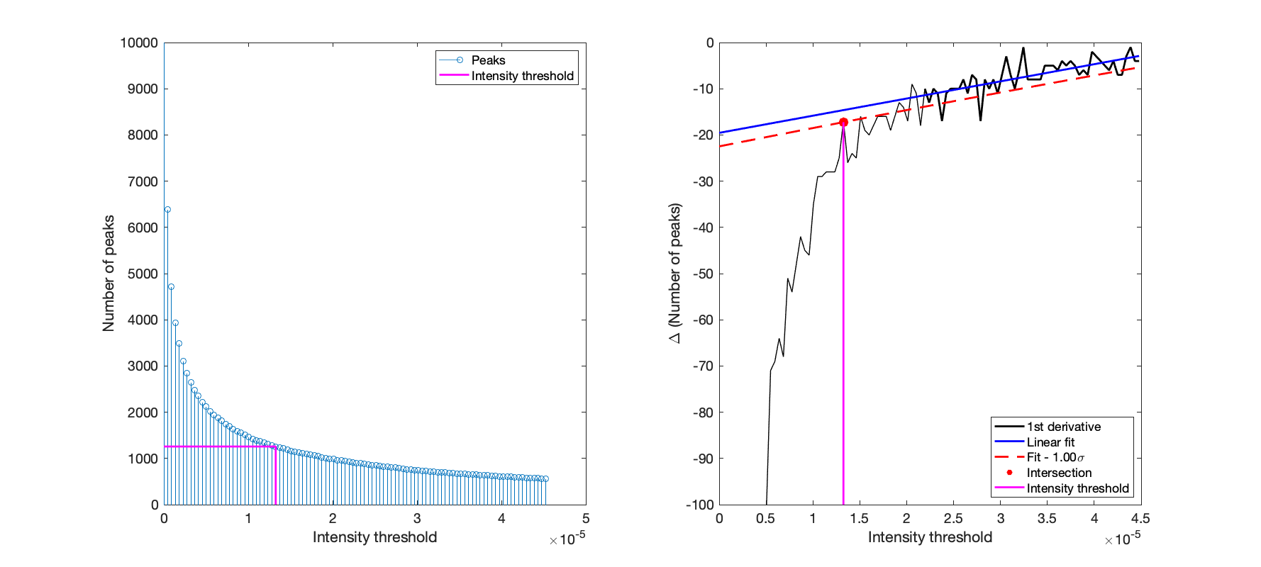 The plot above shows how the number of peaks is determined by identifying a threshold at which peaks are considered to be noise. Essentially the number of peaks is determined at a range of noise thresholds and this is plotted as the stems in the left hand panel. The first derivate of this is plotted, i.e. the difference in the number of peaks for each intensity threshold, which is the black line in the right hand figure. The second half of this data, considered to represent a low rate of change of the number of peaks, is used to fit a linear model which is then extrapolated over the full intensity range. The intersection between the dashed red line and the first derivative is taken as the noise/peak intensity threshold, which is drawn in both axes as the purple line. The red dashed line
 multFac times the standard deviations away from the linear fit; thus a larger multFac lowers the dashed red line and hence leads to more peaks being included. Smaller values (towards zero) raise this line and result in a lower number of peaks being selected.
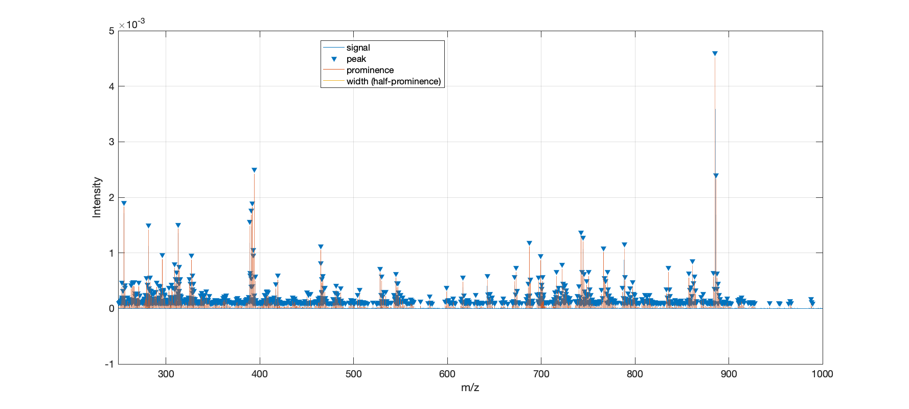 This plot (above) is the standard output figure from the peak picking function. It plots the mean spectrum determined from all files, and the threshold to differentiate noise from genuine peaks is determined based on the figure above.
§4 - Extract these variables from the imzml files
The peaks that were identified from the average spectrum now need to be extracted from the raw data in order to generate a data cube for each file. This is an intensely long process (approximately 10 minutes for centroid mode data, >20 for profile mode data) so should be scheduled overnight if at all possible.
The .mat files that are saved from this analysis are ready for brief statistical analysis such as principal components analysis. For deeper analysis, the optical H&E image with annotations will need to be coregistered to the MS image.
Parameters
recalPath: previously specified output location from the recalibration function
extrPath: a new location into which to save the results
ppmTol = 30: tolerance, ± ppm, for extracting peak intensities from the spectra. This represents the window size around the peak picked m/z value for finding peaks in each pixel’s spectrum
dataType = 'centroid' or 'profile': important to specify due to the way peaks are identified
§5 - Perform PCA
This function will perform an initial combined PCA of all of the images saved in ‘extrPath’. This could be far too many for all of the pixels to be read into computer memory, so to circumvent this the second input to the function is the sampling rate which is used to select a (small) proportion of pixels from each file to be used in performing the PCA. The loadings are then used to project the scores of all of the pixels. Whilst this approximation of PCA is substantially quicker than performing PCA with all pixels across all images, it is still slow enough because it requires the data cubes to be individually loaded to extract the subsampled pixels. Then the PCA is determined which can also be lengthy. And finally the data cubes are loaded individually again and the pixels are projected into this new PCA space. Each file needs to be projected and then the results are output as a variable for use in §6.
Parameters
extrPath: where the extracted datacubes are saved
pcaSamplingRate = x: where x is a numeric value either:
0 < x <= 1: a fractional value to determine how many pixels from each file are used to generate the PCA model. Note that this will result in files contributing unequal numbers of pixels. Ifx = 1then all pixels from all files will be (attempted to be) used1 < x <= maxPix: a positive integer to specify a fixed number of pixels from each file. These pixels will be evenly spaced from the first to the last pixels of the image. As they are not selected randomly, the results will be consistent
Output
The projected PCA scores for each file, which are then visualised in §6.
§6 - Visualise the results from PCA
Plot the results from the previous section. The input parameter numIndividualComponents (integer value from 0 to 10) determines which components are plotted:
numIndividualComponents = 0: plot just the RGB composite image of components 1, 2 and 3numIndividualComponents = 3: plots the first three components as individual images in addition to the RGB imagenumIndividualComponents = 10: a maximum of 10 components are calculated in §5 so 10 is the maximum
Results
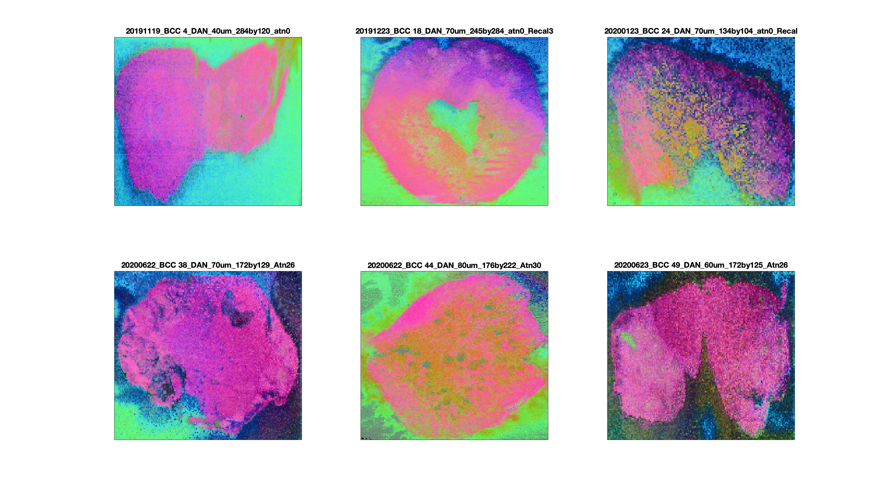 PCA results showing components 1-3 as a series of RGB images. The first component (red) typically differentiates between the tissue and background, as would be expected, and this trend is common across all 6 of the images shown here.
Home-Download-Recalibrate-Pre-process-Annotate1-Annotate2-Coregister-Statistics